I will post here, in this blog, a series of 5 different (sequential) posts for deep technical understanding of “column-oriented dictionary-encoded in-memory database” and its application in enterprise computing.
Part of the content is based on the lecture of the book A Course in In-Memory Data Management – The Inner Mechanics of In-Memory Databases by Hasso Plattner and also based on other researching material available on Google searching, SAP Help and others online learning sources.
I will try to summarize in those posts the 300 pages of the book plus all other lectures and several hours of videos, classes and training (including the Online training presented by Hasso Plattner and also by Dr.-Ing. Jürgen Müller). I will also add some of my own touch and personal understanding and try to make it an “easy understanding” lecture.
I used the learning map presented in the book as a reference to write this and the following posts and in the end I should have covered the following items:
I – The Future of enterprise computing
- New Requirements for Enterprise Computing
- Enterprise Application Characteristics
- Changes in Hardware
- Blueprint SanssouciDB
II – Foundations of database storage techniques
- Dictionary Encoding > Compression
- Data Layout > Row, Column, Hybrid
- Partitioning
III – In-memory database operators
- Insert, Update, Delete
- Scan Performance
- Tuple Reconstruction
- SELECT
- Materialization Strategies
- Parallel Data Processing
- Indexes
- JOIN
- Aggregate Functions
- Parallel SELECT
- Workload Management
- Parallel Join
- Parallel Aggregate Functions
IV – Advanced database storage techniques
- Differential Buffer
- Insert-Only Time Travel
- Merge
- Logging – Recovery
- On-the-fly Database Reorganization
V – Foundations for a new enterprise application development era
- Application Development
- Implications
- Dunning
- Views
- Handling Business Objects
- ByPass Solution
As this is the “Part I”, this post is focused on the Chapter I listed above. So, let’s get started.
I – The Future of Enterprise Computing
1. New Requirements for Enterprise Computing
All of us are used to the speed of Google… why? Because it is fast. It doesn’t make sense to use other search engines when Google is simple and fast. We expect the same concept to the Future of Enterprise Computing.
Let’s visualize 2 examples of applications that needs to read massive data from sensors:
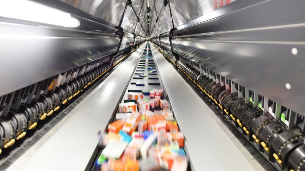
– A Pharmaceutical Industry in Europe:
- Tracking 15 billion packages / 34 billion read events per year
- Distributed repositories for storing read events
- References to read events are stored in central discovery service
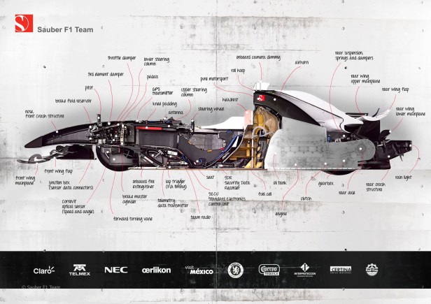
– An application that read sensor’s data from Formula 1 racing cars*:
- Each car has between 300 and 600 sensors
- Multiple events are read per second, per sensor, per car
- Every Grand Prix has around 2 hours of durations and there are 20 per year
- A single car in all 20 races can produce between 43 and 86 billion events to be read and all the cars in the grid will produce between 800 billion and 1.728 trillion events to be captured by those sensors
How to efficiently read and understand all those data? Can the teams predict how the race will end? Can the teams react to the sensor’s data and design a different racing strategy?
Check here to know more how McLaren is using the technology of sensons and big data to improve their car’s performance and predict how the race will end: ‘The biggest science project on the planet’ was on a racetrack on Sunday
Let’s see 2 more examples, this time working with a combination of Structured and Unstructured Data (different file’s formats, manual written notes, etc.):
– Boeing Airplane Maintenance:
- Maintenance workers write reports after each repair
- Every report mentions the part numbers replaced or repaired and they are indexed
- Analytics reveal which parts in other planes may be defective or could become damaged after certain period

– Medical Diagnosis in a huge and connected health system:
- Doctors writ medical reports after every diagnosis
- Diagnosis, symptoms, drugs and reaction to them are indexed
- Comparison with similar cases can suggest what would be the optimal treatment

In all those 4 scenarios, we are dealing with a huge amount of data, in some cases it can help companies been more profitably or cost efficient (in the pharmaceutical industry or in the formula 1 racing for example) and in others it can help saving lives (in the airplane maintenance or medical treatment).
All the data holds huge amount of knowledge and information and processing them, storing the data and could perform effective analysis was a challenge due to technology restrictions (hardware, database layout etc.). It is not anymore… The technology boundaries were broken and we are living a Digital Transformation where AI, Machine Learning, Big Data, IoT and other technologies are enabling companies and segments to rethink their business in a way never seen before.
2. Enterprise Application Characteristics
How do the Enterprise Application use the database?
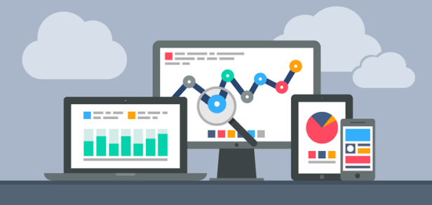
The data base for enterprise applications must serve many different applications, like transactional data entry where you enter orders, invoices etc., data coming into the system. Then we have real-time analytics and structured data: people want to have access to reports that will tell how much they sold, the predictions for next quarter, how are the profits comparing to the same period in the year before. Then we have event processing, streaming data, like the sensor’s examples above, reading events from machines. Enterprise also wants to analyze what happens on Twitter or Facebook (and others social media), and do sentiment analysis of their public, that’s done in text analytics and unstructured data, then you can react to the mood of your customer. If there are discussions going on at Twitter and you don’t see that and don’t comprehend it in a week or a month, your company’s reputation is already damaged.

OLTP vs. OLAP
There are two different types of work that a database can do to your company’s application: Transactional and Analytical.
The transactional and analytical queries are different in some spheres but they are nearly the same in other characteristics. Transactional Queries in the OLTP system (Online Transaction Processing) can be performed entering sales orders in the system, billing documents, posting accounts receivable, displaying a single document entered in the system or checking a single master data while in the OLAP system (Online Analytical Processing) it is all about analysis of the transactional data like reporting, sales forecast, payment reminders, potential cross selling (a sales person can identify opportunities to selling additional services or products to a customer based on information of his Social Network interests for example).
The data system landscape (DBMS) was built and designed to handle the OLTP and OLAP queries separately as the execution time of OLAP queries are higher than OLTP. Then analytical processing tends to affect performance of daily business that are core processes to the company, like manufacturing and selling. So, the enterprise management systems are optimized either to OLTP or OLAP workload because of performance. Because the performance of the analytical application was too slow, those systems were split, and then the company had to extract data from their transactional systems (OLTP) to a system that was optimized for analytical processing (OLAP).
It was always considered that the workload on OLTP was write intensive (because of all the data-entry in transactions) while OLAP was ready-only (because it is only reporting), however, recently research in multiple companies shows that this is not true.
Those researches showed also that the lookup rate in an OLTP system is only 10% higher than OLAP and the number of inserts is a little higher on OLTP, but OLAP systems also deals with inserts as they need to keep the data updated based on what is been performed in the transactional system. It is also known now that the number of updates in OLTP system is not too high as it did believe. In most of the industries with an updated management system the updated on OLTP represents 12% which means, 88% of the rows stored in OLTP are never updated. Those information leads to a new approach on deleting and inserting records in the database and combine the two systems in one.
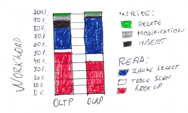
83% of the workload on OLTP are read queries which makes sense, you don’t just enter data, but you want to do something with the data, like reading the invoice data before sending the physical invoice to the customer and only 17% of the workload are writing queries.
In OLAP system you have a bit more read queries but the difference is very low. So, why not using the optimization done in OLAP for read optimize, and use that in OLTP system as well? And that’s where the Column Oriented system comes in place, which was possible due to the modernization on hardware area, creating then a single source of truth for real-time analytics, doing everything on the fly and removing aggregates.
The main difference between OLTP and OLAP is that in the OLTP system, a single select deals with more queries returning only few rows results while OLAP calculate aggregations for few columns of a table but returning many rows. To keep the OLAP and OLTP systems updated and synchronized, it is required a huge ETL (Extract, Transform and Load) process which takes time and it is complex to extract the data and make it fit in the analytical format.
The Disadvantage on separate OLAP from OLTP
It is true that keeping OLAP and OLTP in separated system optimize workload performance to both, but in other hands, there are some disadvantages, such as:
- OLAP will never have the latest updated data as the time to refresh data between the two systems can range from minutes to hours, so many decisions taken based on reports will have to rely on “old” data instead real-time data. Think about in a marketing campaign that needs to be analyzed based on the mood of your customers analyzing what they are saying on Twitter. The number of tweets goes over 350,000 tweets per minute, so, what is happening out there can change in minutes.
- To have an acceptable performance, OLAP system needs to use materialized aggregated, reducing the flexibility of the reporting to different user’s needs.
- OLTP and OLAP schemas are very different, then the applications that use both requires a complex ETL process to keep the data synchronized.
- Usually, not ALL the transactional data is exported to the analytical system, but only a predefined subset of the data (some fields that will be used to report A, B or C) which leads to redundancy, for example, some of the data on Report A is also on C but not or B and some of the data of report B is on A but not on report C.
What can be changed?
It was possible to identify through research on companies’ systems behavior that many fields in a table is not used while those tables get wider and wider. Roughly, more than 50% of the columns are not used in tables where hundreds of columns exist. Among of the columns used there are few distinct values in them, and the other columns are full of NULL or default values, they are not used even once, so those tables contents are very low, near to zero.
By identifying those characteristics, it is possible to think about compression techniques which results in lower memory / data consumption.
After analyzing financial accounting header documents across multiple industries, such as Consumer Packed Goods, Logistics, Banking, High-Tech and Discrete Manufacturing, it was observed that, although those documents had 99 fields, only a small number of columns had a huge number of distinct values (usually the primary key columns), few columns with 10% to 30% distinct values and then many fields that is not used even once.
Overall, comparing Inventory Management and Financial Accounting, across those companies, most of the columns only have 1 to 32 distinct values:

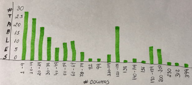
In addition to that, looking to tables (144 most used tables in an ERP system – large number of records), it was analyzed how many columns those tables have. You will see there are 26 tables with few columns (1 to 9), but there are tables with more than 120 columns , and tables with more than 200 to almost 400 colums… How to make those tables more efficient?
3. Changes in Hardware

Up until 2002, hard disk drives used the same basic technology as the old IBM RAMAC.
2017 – SD Card and Micro SD 1 Terabyte


Hardware enabling rethink

A quick view on Memory Hierarchy
We are now talking about a Database system that was optimized to work in main memory as the primary persistence, no longer using Flash Disk or the bloody spinning disks (Hard Drive), they are only used for recovery.
The systems are now also optimized to CPU Caches access (Cache L1, L2, L3), where the “computing” happens.

Years ago, memory was very expensive, and for this reason, only small amounts of memory were available across the company’s servers. The limitation on memory was an obstruction in the data flow from Hard Drive to CPU. The CPU was always idle waiting for the data to arrive through a narrow gateway.
With memory been more accessible, prices dropping, huge amounts of memory are available in the companies, terabytes of them, that made possible to rethink how data would flow to CPU, eliminating the existing waiting times. Following the fact that huge memory becomes available, processor’s industry improved at an extraordinary rate, with high speed multi-core processors allowing the most complex tasks to be processed in parallel, carrying out real-time elaborated analytical tasks, such as predictive analysis and only “memory” can provide data to CPU very fast.

Taking ERP applications that were written along of the past 20 years and making them work in the new hardware wasn’t an option. It would have some gain for sure, but the classic database as we know and the applications, were designed over a restricted hardware architecture, that means, they would not be able to explore the maximum power of the new hardware.
That was when SAP (lead market in ERP systems) decided that the database would have to be reinvented and the HANA database started to be designed.
Latency Numbers

Reading data from CPU L1 Cache to the CPU core takes only 0.5ns while referencing data from Main Memory, that will be loaded through cache hierarchy to the CPU core takes 100ns, which is fast but it is 200 times slower than the CPU L1 Cache.
The time necessary to get data to the core processing is longer as it gets away from the core. That means, Hard Disk is the work-performer by a big significant amount of time. Seek data in the Hard Disk is 100,000 slower than referencing data from main memory and 20 million times slower than L1 CPU cache!!!
That is a good reason to, if you can, keep all the data in Main Memory, not in Disk.
But what is a nanosecond?
According to Wikipedia, A nanosecond (ns) is a SI unit of time equal to one billionth of a second (10−9 or 1/1,000,000,000 s). One nanosecond is to one second as one second is to 31.71 years. A nanosecond is equal to 1000 picoseconds or 1⁄1000 microsecond. Because the next SI unit is 1000 times larger, times of 10−8 and 10−7 seconds are typically expressed as tens or hundreds of nanoseconds.
So, a nanosecond is fast, very fast and it is how processor speeds need to perform for modern application in a digital economy.
Here is another way to read it, with some extra numbers for scale:

For many years disk access has been pushed to the limit and now performance become restricted by the basic physics rules of the spinning disk.
Modern CPU processors are built with CPU cache in layers, which allows managing on-board memory in a very efficient way.
SAP spent the last year working closely with CPU manufacturers in product’s co-development projects to understand better how to explore and make maximum efficient usage of all the power from their processors, understanding how data moves from memory to core.
Because main memory is volatile, hard disks are still needed for now, for logging and backups but eventually even that will go away in favor of other technologies such as SSD (Solid State Drive).
4. A Blueprint of SanssouciDB
SanssouciDB is a visionary database system designed for serving ERP transactions and analytics out of the same data store. It consists of a column-store engine for high-speed analytics and transactions on sparse tables, as well as an engine for so-called combined columns, i.e., column groups which are used for materializing result sets, intermediates, and for processing transactions on tables touching many attributes at the same time, optimized to run In-Memory Database.
Main Memory is non-persistence memory, that is, when the system is shutdown, the data in main memory is lost. To deal with that, the In-Memory Database it is still doing logging and recovery from hard disk, to store and load the data from memory to disk and from disk to memory.
As explained in the “hardware” session, the Hard Disk is not the bottleneck anymore, but the Main Memory, which is 100 times slower than the CPU L1 Cache. Because of that, the DB algorithms should be cache-conscious to get the data from Main Memory and cache it to the CPU Core as fast as possible.
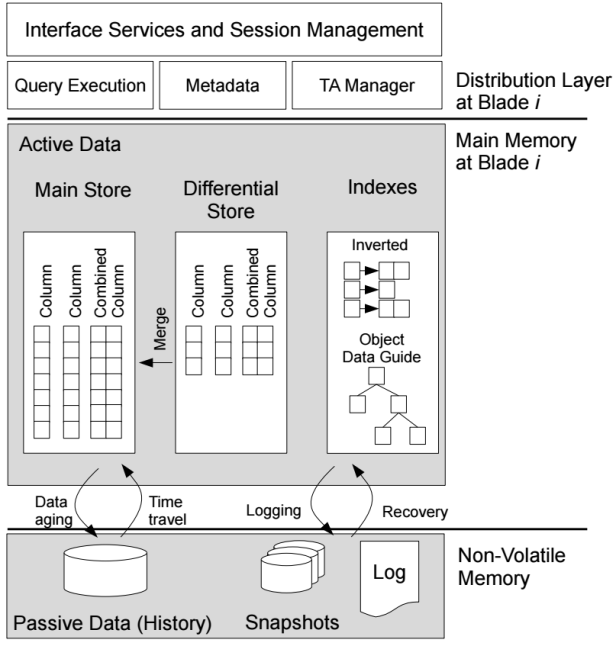
The new system has the Main Store, with the column organized data and there is also the Differential Buffer which is merged from time-to-time into the Main Store.
Indexes can be used, but they are not required as the main store is column-oriented without aggregates, already fully indexed.
Snapshots of the main memory data are done from time-to-time to non-volatile memory (hard-disk) and logging will guarantee the perfect restore when the system is shutdown.
It ends here the Chapter I – The Future of enterprise computing. in the next post, the “Part II” will cover the items listed on the begin of this post for the Chapter II – Foundations of database storage techniques.

Nice blog right here! Also your site loads up fast! What host are you using? Can I get your associate link to your host? I want my site loaded up as quickly as yours lol
LikeLike