In-Memory Data Management – Part II

This post is a sequence of In-Memory Data Management – Part I.

In this post, I will cover the Chapter 2 of the learning map showed in my previous post, which covers the following:

II – Foundations of database storage techniques

1. Dictionary Encoding > Compression
2. Data Layout > Row, Column, Hybrid
3. Partitioning

Without further ado, let’s start…

1. Dictionary Encoding > Compression

Since the CPU is much faster than memory, the memory is now the new bottleneck, as hard disk is no longer used to fetch data to the CPU.

The Dictionary Encoding is a compression technique that decreases the number of bits used to represent data and therefore, reduce the number of operation to get the data from main memory to CPU, enhancing system speed performance.

The dictionary encoding is the foundation to many other compression techniques which can be performed over encoded columns. This is achieved reducing the redundancy by replacing occurrences of values with shorter reference of those values by using the value dictionary and attribute vector. This default method of compression is applied to all columns. Later we can review a little more about compression, but first, let’s focus on the Dictionary Encoding over columns store.

Dictionary encoding is simple. It doesn’t mean that it is easy to learn, but it is easy to implement.

To those who have researched online or read Prof. Hasso Plattner documentation before reading this documentation, you know that I will use the world population as an example. It may sound repetitive, but it easy to general understanding.

The dictionary encoding works column-wise, so let’s assume that the world’s population is 8 billion people (it is actually 7.51B in July 2017 and expected to be 9.6B in 2050). Now let’s imagine a table with the following fields:

• First Name (fname)
• Last Name (lname)
• Gender (gender)
• Country (country)
• City (city)
• DOB (birthday)

Dictionary Encoding – Column

In the Dictionary Encoding, each column splits into 2 columns:

Dictionary – Will store all distinct values (atomic values) that appears in the column, each of them with a valueID (position). The dictionary can be unsorted or in sorted order (which allows fast interaction and it is good for inserts and joints).

Attribute Vector – Will have all ValueIDs to all entries in the column. The valueID encodes the actual value that was recorded in the column. The valueID will repeat as many times as a distinct value appears in the column. We replace the String by an Integer to represent that String as the Attribute Vector points to the dictionary via valueID.

Note that in the attribute vector, the valueID 33 appears twice (to the recIDs 59 and 62). That’s because in the column fname from our world_population table, James appears twice. The more often identical values appear, the greater are the compression-benefits.

The advantage of having a dictionary and an attribute vector to each column is that we only need a few number of bits to encode the fname, as there is low cardinality in the fname column (among 8 billion first names, the repetition is huge) and it is not needed to write all the characters of the fname every time a first name repeats. Modern CPU processors can calculate and build the output information very fast using the ValueID and recID (the relative position in the table).

How to retrieve the data then?

Let’s say our query is to list all humans in the world where the first name is Michelle in a database where it is dictionary encoded.

1. The first thing to do is to scan the dictionary’s value searching for Michelle to retrieve the corresponding valueID. In this example, Michelle is represented by the valueID 34.
2. Then we go to the attribute vector and scan all positions assigned to the valueID 34.
3. Then to output the results, it just replaces the valueID 34 in all positions found, by the respective value in the dictionary (Michelle in this case).

Dictionary entries are sorted either by their numeric value or lexicographically.

Compression Data Size Example with Data Dictionary

Each entry in the world_population table are represented with 200 Bytes:

The total size of world_population tables without data dictionary compression is:

8 billion rows * 200 Byte = 1.6 Terabytes

Encoding the fname column using the binary logarithm (log2) requires only 23 bits to store all the 5 million distinct names in the attribute vector [log2(5,000,000)] = 23.

Then instead using 8 billion * 49 Bytes = 392 billion Bytes = 365.1 GB to store the fname column, the attribute vector can be reduced to 8 billion * 23 bits = 184 billion bits = 23 billion Bytes = 21.4 GB and to the dictionary will need 49 Byte * 5 million = 245 million Byte = 0.23 GB.

The compression results are 21.4GB + 023GB, which is approximately 17 times shorter than the 365.1GB when the compression encoding technique is not applied.

Now, let’s see the compression of column gender which has only 2 distinct values, “m” or “f”.

The data without compression is 8 billion * 1 Byte = 7.45 GB while using the compression, the attribute vectors will take 8 billion * 1 bit = 8 billion bits = 0.93 GB and the dictionary will take 2 * 1 Byte = 2 Bytes.

The compression results are 0.93GB + 2 Bytes which is approximately 8 times shorter than the data without compression, 7.45GB.

Comparing fname and gender we realize that the compression rate depends on the size of the initial data but also the number of distinct values and table cardinality.

The most important effect in dictionary encoding is that all operations concerning table data are now done via attribute vectors and this brings a huge improvement on all operations as CPU were designed to perform operations with numbers, not with characters.

Let see in more details the overall compression in the whole world_population table:

First names – It was found about 5 million different first names. We need 23 bits to encode them (with 1 bit we can encode 2 different values, 2 bits can encode 4 different values, 3 bits can encode 8 different values, 4 bits can encode 16 different values and etc.).

Note: 1 bit can either be 1 or 0, that’s 2 values. 2 bits, which can either be 00, 01, 10 or 11, that’s 4 values, and so on and so forth.

It was assumed to this experiment that the longest first name size is 49 characters long, then it was reserved 49 bytes to first names.

Without using the dictionary encoding compression, it is necessary 365.10 Gigabytes to hold all the 8 billion first names.

In the compressed scenario, we will have 2 data structures, the Dictionary that will hold the atomic values, 5 million first names require 234 MB and the attribute vector with 8 billion entries, each entry with the size of 23 bit required to hold the valueID and the attribute position, a total of 21.42 GB

In summary, just for first names, without dictionary encoding it is required 365.10 GB and with dictionary encoding: 21.65 GB, the compression factor is about 17.

By applying the same technique in all the 6 columns and 8 billion rows of world_population table, the size required to storage the data is about 92 GB while without the compression, it is necessary 1.5 TB!!!

The message here is that the dictionary encoding will allow to handle “less” data, therefore speeding up the processing time required to retrieve the same results with compression, since less data is passed from memory to CPU.

 

2. Data Layout – Row, Column, Hybrid

As the name random access memory suggests, the memory can be accessed randomly and one would expect constant access costs. Main memory is one dimensional structure that can be accessed in different ways. Data can be fetch from memory in a sequential array or random array. Benchmarks proof that the performance of main memory accesses can largely differ depending on the access patterns and to improve application performance, main memory access should be optimized to exploit the usage of caches, as the larger the accessed area in main memory, the more capacity cache misses occur, resulting in poor application performance. Therefore, it is advisable to process data in cache friendly fragments if possible.

To help illustrate this situation, let’s consider the sequential and the random array methods to represent a relational table in memory and assume that all the data stored in this table is “string” data type.

The database must transform its two-dimensional table into a one-dimensional series of bytes for the operating system to write them to memory. The classical and obvious approach is a row based layout. In this case, all attributes of a row are stored consecutively and sequentially in memory: ‘‘1, John Jones, Australia, Sydney; 2, Bryan Quinn, USA, Washington; 3, Lauren Falks, Germany, Berlin’’.

It will be the opposite in a column based layout where the values of one column are stored together, column by column, instead row by row: ‘‘1, 2, 3; John Jones, Bryan Quinn, Lauren Falks; Australia, USA, Germany; Sydney, Washington, Berlin’’.

Column-store is more efficient for reading data from memory, as it is useful to retrieve data from many rows but only on a smaller subset of all columns, since the values of a given column can be read sequentially. The classical row-based is more efficient when performing operations in single records or inserting new records. That’s why row-oriented is used for OLTP data processing and column-store is used in data warehouse on OLAP scenarios.

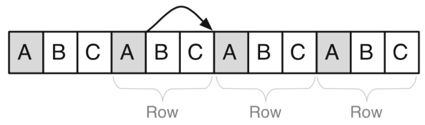
In a row data layout, you can think like an excel sheet where you store your data to the first row 1, then the second data to the following row 2 and so on. While in a column layout is the other way around, where you will store all values of the first column A consecutively, then all value of your second column B and so on.

Row Data Layout

In row data layout, data is stored row-wise and it has a low cost for reconstruction, but higher cost for sequential scan of a single attribute.

In the world_population table, we would have habitants of the world behind each other. If I want to retrieve James then I can go to the row where James is stored and get his first name, last name, gender, city and birthday… While in a column operation, if I want to count how many Male or Female we have in the world, this is going to be much more complex, because first I need to access Column A, then I must jump to the next record and then to the next, to get all genders.

Column Operation

Row Operation

 

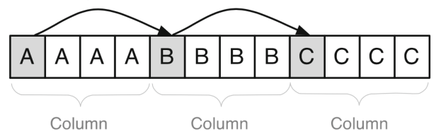
Columnar Data Layout

How it would work in a column data layout to retrieve the same data? It is quite different as the data is stored attribute-wise and not row-wise. Reading data is faster, for example, all habitants with first name James would be stored together, all Male genders then would be stored together after the name and so on and so forth. So, it is very easy to scan through the values and retrieve the data. But in a row operation, when I need to retrieve all data for James, last name, gender, city, birthday etc., then we will have to jump between the columns.

Column Operation

Row Operation

As mentioned more above, there will be use cases where a row-oriented table layout can be more efficient, however, the many advantages speak in favor of columnar layout in an enterprise scenario.

When analyzing the workloads enterprise databases are facing, it turns out that the actual workloads are more read-oriented and dominated by set processing.

Additionally, despite the fact that hardware technology develops very rapidly and the size of available main memory constantly grows, the use of efficient compression techniques is still important in order to keep as much data in main memory as possible and to minimize the amount of data that has to be read from memory to process queries as well as the data transfer between non-volatile storage mediums and main memory.

Using column-based table layouts enables the use of efficient compression techniques. Dictionary encoding can be applied to row-based as well as column-based table layout, whereas other techniques like prefix encoding, run-length encoding, cluster encoding or indirect encoding directly leverage the benefits of columnar table layouts.

Finally, columnar layouts enable much faster column scans as they can sequentially scan the memory, allowing on the fly calculations of aggregates and the result of it is that storing pre-calculated aggregates in the database can be avoided, minimizing redundancy and complexity of the database.

 

Hybrid Data Layout

Each commercial workload is different and might favor a row-based or a column-based layout. The Hybrid table layouts are a mix of both row and column based that combines the advantages of both layouts, allowing to store single attributes of a table column oriented while grouping other attributes into a row-based layout. The actual optimal combination highly depends on the actual workload and can be calculated by layouting algorithms.

For example, imagine attributes, which may belong together in commercial applications, for example quantity and unit of measure or payment terms and payment conditions in finance. The concept of hybrid layout is that if the set of attributes are processed together, it makes sense from a performance standpoint, to store them also together. Considering the table with 3 entries listed above and assuming the fact that the attributes Id and Name are often processed together, we can outline the following hybrid data layout for the table: ‘‘1, John Jones; 2, Bryan Quinn; 3, Lauren Falks; Australia, USA, Germany; Sydney, Washington, Berlin’’.

The hybrid layout may decrease the number of cache misses caused by the expected workload, resulting in increased performance. The usage of hybrid layouts can be beneficial but also introduces new questions like how to find the optimal layout for a given workload or how to react on a changing workload.

3. Partitioning

Data Partitioning is the process of dividing a logical database into distinct independent datasets. It defines the distribution of data in multiple independent and non-overlapping parts and it is an easy way to achieve data-level parallelism, which enables performance gains. It is a technical step to increase query performance-speed.

As partitioning is a classic example of a problem that can’t be solved in polynomial time, the main challenge in this technique is to find the optimal partitioning.

The two main types of data partitioning are: Vertical and Horizontal.

• Vertical partitioning results in dividing the data into attribute groups where typically the primary key is replicated. These groups are then distributed across two or more tables:

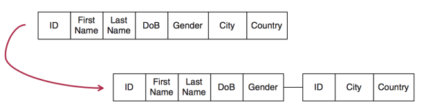
The attributes that are usually accessed together should be in the same table, in order to increase join performance.

While in row-store layout the vertical partitioning is possible, it is not a common approach because it is hard to establish, due to the underlying concept of values row-wise is contradicted when separating parts of the attributes. The column-store layout implicitly supports vertical partitioning, since each column can be regarded as a possible partition.

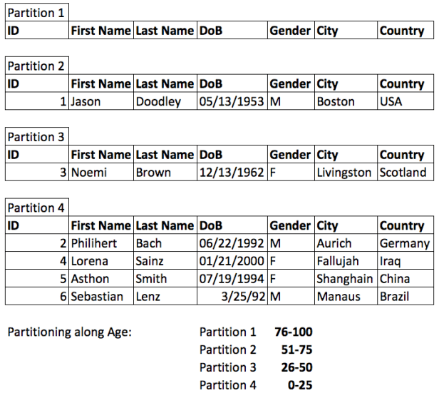
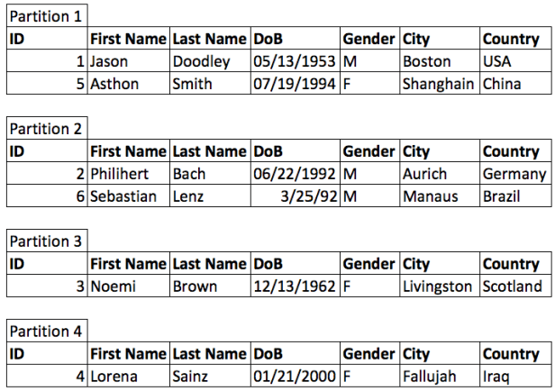
• Horizontal Partitioning is used more often in row-store databases. The table is split into row groups by some condition.

There are several sub-types of horizontal partitioning:

• The first partitioning approach is range partitioning, which separates tables into partitions by a predefined partitioning key, which determines how individual data rows are distributed to different partitions. The partition key can consist of a single key column or multiple key columns. For example, customers could be partitioned based on their date of birth. If one is aiming for a number of four partitions, each partition would cover a range of about 25 years Because the implications of the chosen partition key depend on the workload, it is not trivial to find the optimal solution.

• The second horizontal partitioning type is round robin partitioning. With round robin, a partitioning server does not use any tuple information as partitioning criteria, so there is no explicit partition key. The algorithm simply assigns tuples turn by turn to each partition, which automatically leads to an even distribution of entries and should support load-balancing to some extent

However, since specific entries might be accessed way more often than others, an even workload distribution cannot be guaranteed. Improvements from intelligent data co-location or appropriate data-placement are not leveraged, because the data distribution is not dependent on the data, but only on the insertion order.

• The third horizontal partitioning type is hash-based partitioning. Hash partitioning uses a hash function to specify the partition assignment for each row. The main challenge for hash-based partitioning is to choose a good hash function, that implicitly achieves locality or access improvements

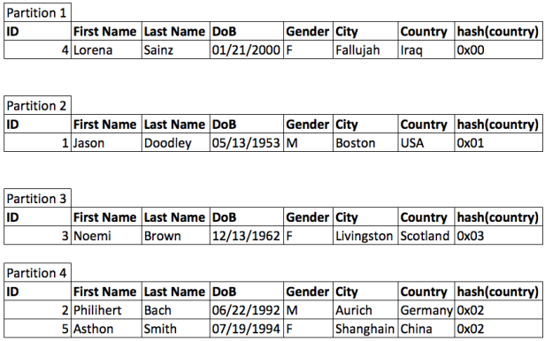
For example: Select an attribute that will be hashed, in the example above, country is used as a starting point to hash-code, but because countries have completely different sizes, it was hashed all the countries to a smaller set of hash keys, then we get a decent balance and we end with fewer hash keys than countries and when we need to input a country the system can calculate a hash key.

• The last partitioning type is semantic partitioning. It uses knowledge about the application to split the data. For example, a database can be partitioned according to the life-cycle of a sales order. All tables required for the sales order represent one or more different life-cycle steps, such as creation, purchase, release, delivery, or dunning of a product. One possibility for suitable partitioning is to put all tables that belong to a certain life-cycle step into a separate partition. The application is the layer that tells if partitioning should be performed in active data only or active and history data. The database can’t figure out it, the database can only provide the splitting.

There are some different optimization goals to be considered before choosing the partitioning strategy that is more suitable and the best partitioning strategy depends very much on the specific use case.

It ends here the Chapter II – Foundations of database storage techniques, in the next post, the “Part III” will cover the items listed on the begin of the post “Part I” for the Chapter III – In-memory database operators.