Dictionary Encoding

With the possibility of replacing hard disk by memory, and since the CPU is much faster than memory, the memory now is the new bottleneck.

The Dictionary Encoding is a compression technique that decreases the number of bits used to represent data and therefore, reduce the number of operation to get the data from main memory to CPU, enhancing system speed performance.

The dictionary encoding is the foundation to many other compression techniques which can be performed over encoded columns. This is achieved by reducing the redundancy by replacing occurrences of values with shorter reference of those values by using the value dictionary and attribute vector. This default method of compression is applied to all columns. Later we can review a little more about compression, but first, let’s focus on the Dictionary Encoding over columns store.

Dictionary encoding is simple. It doesn’t mean that it is easy to learn, but it is easy to implement.

If you have researched online or read Prof. Hasso Plattner documentation before, you know that I will use the world population as an example. It is repetitive, but it better to general understanding.

The dictionary encoding works column-wise, so let’s assume that the world’s population is 8 billion people (it is actually 7.49B in March, 2017 and expected to be 9.6B in 2050). Now let’s imagine a table with the following information:

• First Name (fname)
• Last Name (lname)
• Gender (gender)
• Country (country)
• City (city)
• DOB (birthday)

Here is a sample data of people in this world_population table:

Dictionary Encoding – Column

In the Dictionary Encoding, each column splits into 2 columns:

• Dictionary – Will store all distinct values (atomic values) that appears in the column, each of them with a valueID (position). The dictionary can be unsorted or in sorted order (which allows fast interaction)
• Attribute Vector – Will have all ValueIDs to all entries in the column. The valueID encodes the actual value that was recorded in the column. The valueID will repeat as many times as a distinct value appears in the column.

Note that in the attribute vector, the valueID 33 appears twice (to the recIDs 59 and 62). That’s because in the column fname from our world_population table, James appears twice. The more often identical values appear, the greater are the compression-benefits.

The advantage of having a dictionary and an attribute vector to each column is that we only need a few number of bits to encode the fname, as there is low cardinality in the fname column (among 8 billion first names, the repetition is huge) and it is not needed to write all the characters of the fname everytime a first name repeats. Modern CPU processors can calculate and build the output information very fast using the ValueID and recID.

 

How to retrieve the data then?

Let’s say our query is to list all humans in the world where the first name is Michelle in a database where it is dictionary encoded.

1. The first thing to do is to scan the dictionary’s value searching for Michelle to retrieve the corresponding valueID. In this example, Michelle is represented by the valueID 34.
2. Then we go to the attribute vector and scan all positions assigned to the valueID 34.
3. Then to output the results, it just replaces the valueID 34 in all positions found, by the respective value in the dictionary (Michelle in this case).

Compression Example with Data Dictionary

Each entry in the world_population table are represented with 200 Bytes:

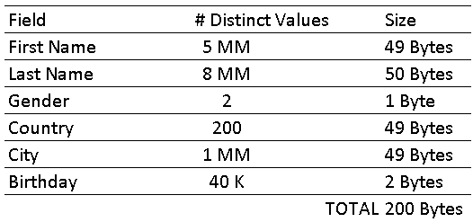
The total size of world_population tables without data dictionary compression is:

8 billion rows * 200 Byte = 1.6 Terabytes

Encoding the fname column: using the binary logarithm (log₂) we know that only 23 bits are required to store all the 5 million distinct names in the attribute vector [log₂(5,000,000)] = 23.

Then instead using 8 billion * 49 Bytes = 392 billion Bytes = 365.1 GB to store the fname column, the attribute vector can be reduced to 8 billion * 23 bits = 184 billion bits = 23 billion Bytes = 21.4 GB and the additional dictionary will need 49 Byte * 5 million = 245 million Byte = 0.23 GB.

The compression results are 21.4GB + 023GB, which is approximately 17 times shorter than the 365.1GB when the compression encoding technique is not applied.

Now, let’s see the compression of column gender which has only 2 distinct values, “m” or “f”.

The data without compression is 8 billion * 1 byte = 7.45 GB while using the compression, the attribute vectors will take 8 billion * 1 bit = 8 billion bits = 0.93 GB and the dictionary will take 2 * 1 Byte = 2 Bytes.

The compression results are 0.93GB + 2 bytes which is approximately 8 times shorter than the data without compression, 7.45GB.

Comparing fname and gender we realize that the compression rate depends on the size of the initial data but also the number of distinct values and table cardinality.

The most important effect in dictionary encoding is that all operations concerning table data are now done via attribute vectors and this brings a huge improvement on all operations as CPU are designed to perform operations with numbers, not on characters.

Let see in more details the overall compression in the whole world_population table, check it out:

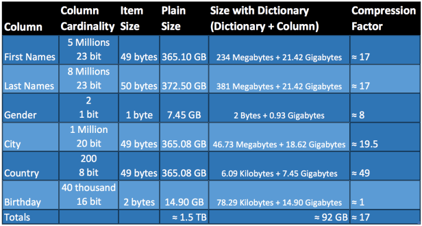
First names – It was found about 5 Million different first names. We need 23 bit to encode them (with 1 bit we can encode 2 different values, 2 bits can encode 4 different values, 3 bits can encode 8 different values, 4 bits can encode 16 different values and etc.).

Note: 1 bit can either be 1 or 0, that’s 2 values. 2 bits, which can either be 00, 01, 10 or 11 That’s 4 values, and so on and so forth.

It was assumed to this experiment that the longest First Name size is 49 characters long, then it was reserved 49 bytes to first names.

Without using the dictionary encoding compression, it is necessary 365.10 Gigabytes to hold all the 8 billion first names.

In the compressed scenario, we will have 2 data structures, the Dictionary that will hold the atomic values, to hold 5 million first names, it is necessary 234 MB and the attribute vector will have 8 billion entries and each entry with the size of 23 bit required to hold the valueID and the attribute position, a total of 21.42 GB

In summary, just for first names, without dictionary encoding it is required 365.10 GB and with dictionary encoding: 21.65 GB, the compression factor is about 17.

By applying the same technique in all the 6 columns and 8 billion rows of world_population table, the size required to storage the data is about 92 GB and without the compression, it is necessary 1.5 TB!!!

The message here is that the dictionary encoding will allow to handle “less” data, therefore speeding up the processing time required to retrieve the same results/data with compression, since less data is passed from memory to CPU.

 

Sources:

• Cache Conscious Column Organization in in-memory column stores – David Schwalb, Jens Krüger, Hasso Plattner
• A Course in In-Memory Data Management – The Inner Mechanics of In-Memory Databases – Hasso Plattner
• The In-Memory Revolution: How SAP HANA Enables Business of the Future – Hasso Platner
• Open HPI
• Open SAP